
Series 1: Integrating Medical Research Into Clinical Reasoning: Exploring Bayesian Analysis as a Complement to Traditional Statistics
Keywords
Statistical Inference, Null Hypothesis, Bayes Factor, Clinical Significance, Statistical Significance
Introduction
Statistical methods are the backbone of evidence-based medicine, yet the debate between clinical and statistical significance persists. Clinical significance reflects the practical impact of research findings on patient care, whereas statistical significance often relies on arbitrary thresholds like p-values. A finding that is statistically significant may not translate into meaningful clinical outcomes, and vice versa. 1 For example, a slight reduction in blood pressure may achieve statistical significance in a large cohort but might lack clinical relevance if it does not reduce morbidity or mortality. The distinction between clinical significance (practical impact) and statistical significance (probability under the null hypothesis) is essential. 2 However, meaningful interpretation of research necessitates a thorough understanding of the statistical analyses employed. There are two main approaches to statistical analysis: frequentist and Bayesian. 3
Frequentist methods, based on null hypothesis significance testing (NHST), calculate the probability of observing the data given the assumption that the null hypothesis is true. This approach treats parameters (e.g., means, proportions) as fixed quantities and uses data to make probabilistic statements about hypothetical repeated samples, employing fixed thresholds such as p-values to determine statistical significance. 4 However, frequentist methods do not account for prior knowledge and provide limited insights into the plausibility of hypotheses. 5
Bayesian methods treat parameters as random variables and combine prior knowledge with observed data to compute posterior probabilities, offering a more flexible and intuitive framework for statistical inference. 5
Before we introduce the bayesian framework, let us understand what are the limitations of NHST frequentist approach where bayesian appraoch provide a better alternative.
Challenges with Frequentist Methods: 1, 2, 6, 7
-
Dependence on Hypothetical Data: P-values depend on the probability of observing the data (or more extreme) if the null hypothesis is true. This involves considering hypothetical repeated samples that are never actually observed. Example: Imagine you're flipping a coin 100 times. You hypothesize the coin is fair (null hypothesis). The p-value tells you how likely it is to get the observed result if you could flip the coin an infinite number of times.
-
Sensitivity to Researcher Intentions (Optional Stopping): NHST requires a fixed sample size. "Optional stopping" (continuing data collection until you get a significant result) inflates the false positive rate. Example: Consider a study on a new drug. If researchers keep adding patients until they see a significant result, the p-value becomes misleading.
-
Lack of Evidence Quantification: A p-value doesn’t quantify the evidence for or against a hypothesis. It just indicates how unlikely the observed data is under the null hypothesis. Example: A p-value of 0.04 doesn’t mean there's a 96% chance the treatment works. It just means the observed data is unlikely under the assumption that the treatment has no effect (if the null hypothesis is true).
-
Absence of Direct Hypothesis Comparison: NHST only tells you whether to reject the null hypothesis. It doesn’t compare different hypotheses directly. Example: Suppose you have two treatments for a condition. NHST can tell you if one treatment is effective, but not how the two treatments compare directly.
Introduction to the Bayesian Framework 1, 7, 3
Bayesian theory might seem unfamiliar at first, but its principles align closely with how clinicians already think. For example, when diagnosing a patient, a doctor begins with prior knowledge about common illnesses and symptoms. As tests are performed, this information is updated based on the results, narrowing down the possibilities. Bayesian methods formalize this process by combining prior beliefs (prevalence of diseases) with observed data (test results) to calculate updated probabilities for potential diagnoses.
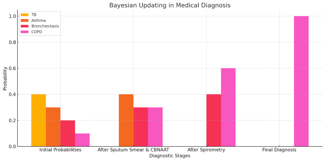
Consider a patient presenting with a chronic cough suggestive of a respiratory condition. Initially, the doctor may suspect tuberculosis (TB), chronic asthma, bronchiectasis, or chronic obstructive pulmonary disease (COPD) with varying probabilities. After sputum smear and CBNAAT tests are performed, if both come back negative, the probability of TB decreases significantly. Additional investigations, such as spirometry and imaging, may then focus on distinguishing between chronic asthma, bronchiectasis, and COPD. As diagnostic tests exclude other conditions, the likelihood of COPD increases. This step-by-step refinement mirrors Bayesian reasoning, ensuring more accurate and evidence-based diagnoses.
The Figure 1 demonstrates Bayesian reasoning in a medical diagnosis scenario. Initially, probabilities are assigned to tuberculosis (TB), asthma, bronchiectasis, and chronic obstructive pulmonary disease (COPD). As diagnostic tests like sputum smear, CBNAAT, and spirometry are performed, probabilities are updated. COPD becomes the most likely diagnosis after ruling out other conditions, illustrating the iterative refinement typical of Bayesian reasoning.
Bayesian analysis offers a robust framework for integrating prior knowledge with new data, providing direct probability statements that align closely with clinical reasoning.
Application of Bayesian A nalysis in Research:
Introducing Bayes Factor 2, 8, 7, 9, 4
Unlike the frequentist approach, Bayesian hypothesis testing is comparative in nature. The likelihood of the data is considered under both the null and alternative hypotheses, and these probabilities are compared via the Bayes factor. The Bayes factor compares the likelihood of the data under the null hypothesis with the likelihood of the data under the alternative hypothesis. It provides a straightforward way to quantify evidence for one hypothesis over the other, allowing researchers to make more informed decisions. In simplified terms:
-
As the Bayes Factor (BF01) increases, there is more evidence supporting the null hypothesis and less favoring the alternative hypothesis.
-
Conversely, if 1/BF01 = 5, this indicates that the data are five times more likely to occur under the alternative hypothesis compared to the null hypothesis.
Instead of simply saying "It is unlikely that there is no relationship between these variables," the researcher can state, "This alternative model is considerably better than the null, and I have the probabilities to prove it!" This allows the inclusion of a statement on how much more likely the data are if the null hypothesis is true compared to if the alternative hypothesis is true. If the prior odds are assumed to be 1, taking the inverse allows one to discuss the likelihood of the alternative hypothesis compared to the null.
For instance, if BF01 = 0.5, the data are half as likely under the null hypothesis as they are under the alternative hypothesis. Taking the inverse shows that the data are twice as likely under the alternative hypothesis. Thus, interpreting a Bayes factor is straightforward, considering those odds.
Several authors (Jeffreys, 1961; Raftery, 1995; Wetzels et al., 2011) 7, 10, 8 have provided guidelines for interpreting Bayes factors.Table 1 summarizes their suggested terminology for discussing Bayes factors, which helps articulate the strength of evidence provided by the data. According to these guidelines, the results could be updated to state that the findings provide such level of evidence for the alternative hypothesis.
|
Bayes Factor (BF01) |
Inverse of Bayes Factor (BF10) |
Raftery (1995) |
Jeffreys (1961) |
|
1–.33 |
1–3 |
Weak |
Anecdotal |
|
.33–.10 |
3–10 |
Positive |
Substantial |
|
.10–.05 |
10–20 |
Positive |
Strong |
|
.05–.03 |
20–30 |
Strong |
Strong |
|
.03–.01 |
30–100 |
Strong |
Very Strong |
|
.01–.0067 |
100–150 |
Strong |
Decisive |
|
<.0067 |
>150 |
Very Strong |
Decisive |
Let us understand the distinct perspectives on statistical inference of both the methods. Suppose we conducted a study comparing two diets' effects on weight loss and found that the frequentist approach, through an independent samples t-test, yielded a barely significant p-value of 0.045. This result suggests a statistically significant difference in weight loss between the groups but leaves uncertainty about the strength of this evidence. On the other hand, a Bayesian analysis of the same data provides a Bayes Factor (BF₁₀) of 2. This indicates that the data are twice as likely under the alternative hypothesis (a difference exists) than under the null hypothesis (no difference between diets), showing weak or anecdotal strength of evidence in support of the alternative hypothesis.
While the frequentist p-value suggests a potential difference, the Bayesian perspective highlights that the evidence for Diet One's superiority is relatively weak. The Bayesian approach offers a more nuanced interpretation by integrating prior knowledge and comparing the probabilities of both hypotheses directly. This comprehensive view underscores the importance of not only identifying statistical significance but also understanding the strength and implications of the evidence in clinical and research settings.
In the next series, we'll explain the procedural steps for conducting Bayesian analysis using JASP software. This will cover data preparation, running the analysis, and interpreting results within a research context. You can begin by downloading JASP from https://jasp-stats.org/download/ . The website offers extensive resources ( https://jasp-stats.org/resources/ ) to help you get started. 9 This series aims to enhance a researcher's proficiency in better analysis of research findings.